Alpha CSC on empirical time-series with strong artifacts#

This example illustrates how to learn univariate atoms on a univariate time-serie affected by strong artifacts. The data is a single LFP channel recorded on a rodent’s striatum 1. Interestingly in this time-serie, the high frequency oscillations around 80 Hz are modulated in amplitude by the low-frequency oscillation around 3 Hz, a phenomenon known as cross-frequency coupling (CFC).

The convolutional sparse coding (CSC) model is able to learn the prototypical waveforms of the signal, on which we can clearly see the CFC. However, when the CSC model is fitted on a data section with strong artifacts, the learned atoms do not show the expected CFC waveforms. To solve this problem, another model can be used, called alpha-CSC 2, which is less affected by strong artifacts in the data.

1: G. Dallérac, M. Graupner, J. Knippenberg, R. C. R. Martinez, T. F. Tavares, L. Tallot, N. El Massioui, A. Verschueren, S. Höhn, J.B. Bertolus, et al. Updating temporal expectancy of an aversive event engages striatal plasticity under amygdala control. Nature Communications, 8:13920, 2017
2: Jas, M., Dupré La Tour, T., Şimşekli, U., & Gramfort, A. (2017). Learning the Morphology of Brain Signals Using Alpha-Stable Convolutional Sparse Coding. Advances in Neural Information Processing Systems (NIPS), pages 1099–1108.

# Authors: Tom Dupre La Tour <tom.duprelatour@telecom-paristech.fr>
#          Mainak Jas <mainak.jas@telecom-paristech.fr>
#          Umut Simsekli <umut.simsekli@telecom-paristech.fr>
#          Alexandre Gramfort <alexandre.gramfort@telecom-paristech.fr>
#
# License: BSD (3-clause)

Let us first load the data sample.

import mne
import numpy as np
import matplotlib.pyplot as plt

# sample frequency
sfreq = 350.

# We load the signal. It is an LFP channel recorded on a rodent's striatum.
data = np.load('../rodent_striatum.npy')
print(data.shape)

Out:

(1, 630000)

Now let us take a closer look, plotting the 100 first seconds of the signal.

start, stop = [0, 100]  # in seconds
start, stop = int(start * sfreq), int(stop * sfreq)
time = np.arange(start, stop) / sfreq
plt.plot(time, data[0, start:stop])
plt.show()

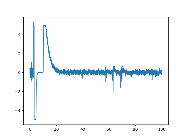
As we can see, the data contains severe artifacts. We will thus compare three approaches to tackle these artifacts:

First, we will fit a CSC model on a section not affected by artifacts.

Then, we will fit a CSC model on a section affected by artifacts.

Finally, we will fit an alpha-CSC model on a section affected by artifacts.

# Define a clean data section.
start, stop = [100, 600]  # in seconds
start, stop = int(start * sfreq), int(stop * sfreq)
data_clean = data[:, start:stop].copy()

# Define a dirty data section (same length).
start, stop = [0, 500]  # in seconds
start, stop = int(start * sfreq), int(stop * sfreq)
data_dirty = data[:, start:stop].copy()

# We also remove the slow drift, which accounts for a lot of variance.
data_clean = mne.filter.filter_data(data_clean, sfreq, 1, None)
data_dirty = mne.filter.filter_data(data_dirty, sfreq, 1, None)

# To make the most of parallel computing, we split the data into trials.
data_clean = data_clean.reshape(50, -1)
data_dirty = data_dirty.reshape(50, -1)

# We scale the data, since parameter alpha is scale dependant.
scale = data_clean.std()
data_clean /= scale
data_dirty /= scale

Out:

Setting up high-pass filter at 1 Hz

FIR filter parameters
---------------------
Designing a one-pass, zero-phase, non-causal highpass filter:
- Windowed time-domain design (firwin) method
- Hamming window with 0.0194 passband ripple and 53 dB stopband attenuation
- Lower passband edge: 1.00
- Lower transition bandwidth: 1.00 Hz (-6 dB cutoff frequency: 0.50 Hz)
- Filter length: 1155 samples (3.300 sec)

Setting up high-pass filter at 1 Hz

FIR filter parameters
---------------------
Designing a one-pass, zero-phase, non-causal highpass filter:
- Windowed time-domain design (firwin) method
- Hamming window with 0.0194 passband ripple and 53 dB stopband attenuation
- Lower passband edge: 1.00
- Lower transition bandwidth: 1.00 Hz (-6 dB cutoff frequency: 0.50 Hz)
- Filter length: 1155 samples (3.300 sec)

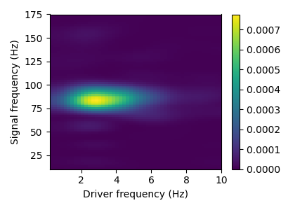
This sample contains CFC between 3 Hz and 80 Hz. This phenomenon can be described with a comodulogram, computed for instance with the pactools Python library.

from pactools import Comodulogram

comod = Comodulogram(fs=sfreq, low_fq_range=np.arange(0.2, 10.2, 0.2),
                     low_fq_width=2., method='duprelatour')
comod.fit(data_clean)
comod.plot()
plt.show()

Out:

[                                        ] 0% | 0.00 sec | comodulogram: DAR(10, 1)
[                                        ] 2% | 0.29 sec | comodulogram: DAR(10, 1)
[.                                       ] 4% | 0.42 sec | comodulogram: DAR(10, 1)
[..                                      ] 6% | 0.54 sec | comodulogram: DAR(10, 1)
[...                                     ] 8% | 0.67 sec | comodulogram: DAR(10, 1)
[....                                    ] 10% | 0.80 sec | comodulogram: DAR(10, 1)
[....                                    ] 12% | 0.93 sec | comodulogram: DAR(10, 1)
[.....                                   ] 14% | 1.06 sec | comodulogram: DAR(10, 1)
[......                                  ] 16% | 1.19 sec | comodulogram: DAR(10, 1)
[.......                                 ] 18% | 1.32 sec | comodulogram: DAR(10, 1)
[........                                ] 20% | 1.45 sec | comodulogram: DAR(10, 1)
[........                                ] 22% | 1.58 sec | comodulogram: DAR(10, 1)
[.........                               ] 24% | 1.70 sec | comodulogram: DAR(10, 1)
[..........                              ] 26% | 1.83 sec | comodulogram: DAR(10, 1)
[...........                             ] 28% | 1.97 sec | comodulogram: DAR(10, 1)
[............                            ] 30% | 2.09 sec | comodulogram: DAR(10, 1)
[............                            ] 32% | 2.23 sec | comodulogram: DAR(10, 1)
[.............                           ] 34% | 2.36 sec | comodulogram: DAR(10, 1)
[..............                          ] 36% | 2.50 sec | comodulogram: DAR(10, 1)
[...............                         ] 38% | 2.62 sec | comodulogram: DAR(10, 1)
[................                        ] 40% | 2.75 sec | comodulogram: DAR(10, 1)
[................                        ] 42% | 2.88 sec | comodulogram: DAR(10, 1)
[.................                       ] 44% | 3.01 sec | comodulogram: DAR(10, 1)
[..................                      ] 46% | 3.14 sec | comodulogram: DAR(10, 1)
[...................                     ] 48% | 3.27 sec | comodulogram: DAR(10, 1)
[....................                    ] 50% | 3.40 sec | comodulogram: DAR(10, 1)
[....................                    ] 52% | 3.53 sec | comodulogram: DAR(10, 1)
[.....................                   ] 54% | 3.66 sec | comodulogram: DAR(10, 1)
[......................                  ] 56% | 3.79 sec | comodulogram: DAR(10, 1)
[.......................                 ] 58% | 3.92 sec | comodulogram: DAR(10, 1)
[........................                ] 60% | 4.05 sec | comodulogram: DAR(10, 1)
[........................                ] 62% | 4.18 sec | comodulogram: DAR(10, 1)
[.........................               ] 64% | 4.31 sec | comodulogram: DAR(10, 1)
[..........................              ] 66% | 4.44 sec | comodulogram: DAR(10, 1)
[...........................             ] 68% | 4.57 sec | comodulogram: DAR(10, 1)
[............................            ] 70% | 4.70 sec | comodulogram: DAR(10, 1)
[............................            ] 72% | 4.83 sec | comodulogram: DAR(10, 1)
[.............................           ] 74% | 4.96 sec | comodulogram: DAR(10, 1)
[..............................          ] 76% | 5.09 sec | comodulogram: DAR(10, 1)
[...............................         ] 78% | 5.21 sec | comodulogram: DAR(10, 1)
[................................        ] 80% | 5.34 sec | comodulogram: DAR(10, 1)
[................................        ] 82% | 5.47 sec | comodulogram: DAR(10, 1)
[.................................       ] 84% | 5.60 sec | comodulogram: DAR(10, 1)
[..................................      ] 86% | 5.73 sec | comodulogram: DAR(10, 1)
[...................................     ] 88% | 5.86 sec | comodulogram: DAR(10, 1)
[....................................    ] 90% | 5.99 sec | comodulogram: DAR(10, 1)
[....................................    ] 92% | 6.12 sec | comodulogram: DAR(10, 1)
[.....................................   ] 94% | 6.25 sec | comodulogram: DAR(10, 1)
[......................................  ] 96% | 6.38 sec | comodulogram: DAR(10, 1)
[....................................... ] 98% | 6.51 sec | comodulogram: DAR(10, 1)
[........................................] 100% | 6.64 sec | comodulogram: DAR(10, 1)

[........................................] 100% | 6.64 sec | comodulogram: DAR(10, 1)

Here we define the plotting function which display the learned atoms.

def plot_atoms(d_hat):
    n_atoms, n_times_atom = d_hat.shape
    n_columns = min(6, n_atoms)
    n_rows = int(np.ceil(n_atoms // n_columns))
    figsize = (4 * n_columns, 3 * n_rows)
    fig, axes = plt.subplots(n_rows, n_columns, figsize=figsize, sharey=True)
    axes = axes.ravel()

    # Plot the temporal pattern of the atom
    for kk in range(n_atoms):
        ax = axes[kk]
        time = np.arange(n_times_atom) / sfreq
        ax.plot(time, d_hat[kk], color='C%d' % kk)
        ax.set_xlim(0, n_times_atom / sfreq)
        ax.set(xlabel='Time (sec)', title="Temporal pattern %d" % kk)
        ax.grid(True)

    fig.tight_layout()
    plt.show()

Then we define the common parameters of the different models.

common_params = dict(
    n_atoms=3,
    n_times_atom=int(sfreq * 1.0),  # 1000. ms
    reg=3.,
    solver_z='l-bfgs',
    solver_z_kwargs=dict(factr=1e9),
    solver_d_kwargs=dict(factr=1e2),
    random_state=42,
    n_jobs=5,
    verbose=1)

# number of iterations
n_iter = 10

# Parameter of the alpha-stable distribution for the alpha-CSC model.
# 0 < alpha < 2
# A value of 2 would correspond to the Gaussian noise model, as in vanilla CSC.
alpha = 1.2

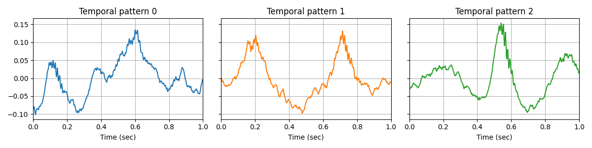
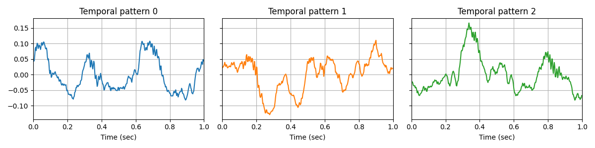
First, we fit a CSC model on the clean data. Interestingly, we obtain prototypical waveforms of the signal on which we can clearly see the CFC.

from alphacsc import learn_d_z, learn_d_z_weighted

X = data_clean

_, _, d_hat, z_hat, _ = learn_d_z(X, n_iter=n_iter, **common_params)

plot_atoms(d_hat)

Temporal pattern 0, Temporal pattern 1, Temporal pattern 2

Out:

V_0/10 .........

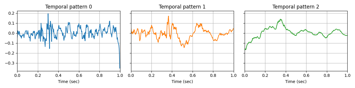
Then, if we fit a CSC model on the dirty data, the model is strongly affected by the artifacts, and we cannot see CFC anymore in the temporal waveforms.

X = data_dirty

_, _, d_hat, z_hat, _ = learn_d_z(X, n_iter=n_iter, **common_params)

plot_atoms(d_hat)

Out:

V_0/10 .........

Finally, If we fit an alpha-CSC model on the dirty data, the model is less affected by the artifacts, and we are able to see CFC in the temporal waveforms.

X = data_dirty

d_hat, z_hat, tau = learn_d_z_weighted(
    X, n_iter_optim=n_iter, n_iter_global=3, n_iter_mcmc=300,
    n_burnin_mcmc=100, alpha=alpha, **common_params)

plot_atoms(d_hat)

Out:

Global Iter: 0/3        V_0/10 .........
Global Iter: 1/3        V_0/10 .........
Global Iter: 2/3        V_0/10 .........

Total running time of the script: ( 11 minutes 40.010 seconds)

Gallery generated by Sphinx-Gallery

Alpha CSC on simulated data

MoTIF on simulated data