Vanilla CSC on simulated data

This example demonstrates vanilla CSC on simulated data. Note that vanilla CSC is just a special case of alphaCSC with alpha=2.

# Authors: Mainak Jas <mainak.jas@telecom-paristech.fr>
#          Tom Dupre La Tour <tom.duprelatour@telecom-paristech.fr>
#          Umut Simsekli <umut.simsekli@telecom-paristech.fr>
#          Alexandre Gramfort <alexandre.gramfort@telecom-paristech.fr>
#
# License: BSD (3-clause)

Let us first define the parameters of our model.

n_times_atom = 64  # L
n_times = 512  # T
n_atoms = 2  # K
n_trials = 100  # N
n_iter = 50

reg = 0.1

Here, we simulate the data

from alphacsc.simulate import simulate_data # noqa

random_state_simulate = 1
X, ds_true, z_true = simulate_data(n_trials, n_times, n_times_atom,
                                   n_atoms, random_state_simulate)

Add some noise and corrupt some trials

from scipy.stats import levy_stable # noqa
from alphacsc import check_random_state # noqa

# Add stationary noise:
fraction_corrupted = 0.02
n_corrupted_trials = int(fraction_corrupted * n_trials)

rng = check_random_state(random_state_simulate)
X += 0.01 * rng.randn(*X.shape)

idx_corrupted = rng.randint(0, n_trials,
                            size=n_corrupted_trials)

Let us look at the first 10 trials to see how they look.

from alphacsc.viz.callback import plot_data # noqa
plot_data([X[:10]])

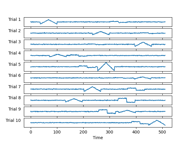
Note that the atoms don’t always have the same amplitude or occur at the same time instant.

Now, we run vanilla CSC on the data.

from alphacsc import learn_d_z # noqa

random_state = 60

pobj, times, d_hat, z_hat, reg = learn_d_z(
    X, n_atoms, n_times_atom, reg=reg, n_iter=n_iter,
    solver_d_kwargs=dict(factr=100), random_state=random_state,
    n_jobs=1, verbose=1)
print('Vanilla CSC')

Out:

V_0/50 .................................................
Vanilla CSC

Finally, let’s compare the results.

import matplotlib.pyplot as plt # noqa
plt.figure()
plt.plot(d_hat.T)
plt.plot(ds_true.T, 'k--')

Out:

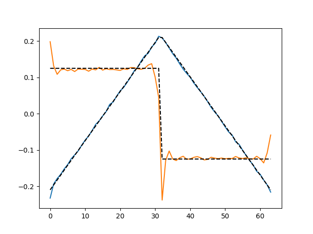
[<matplotlib.lines.Line2D object at 0x7f58a00ac820>, <matplotlib.lines.Line2D object at 0x7f58a00ac850>]

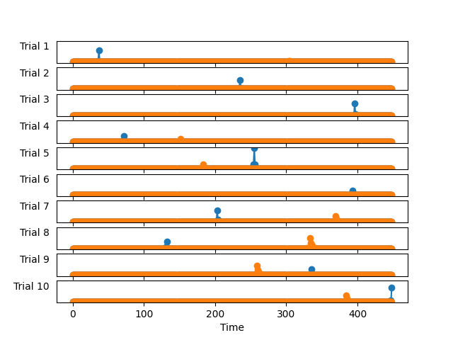
We can also visualize the learned activations

plot_data([z[:10] for z in z_hat], ['stem'] * n_atoms)

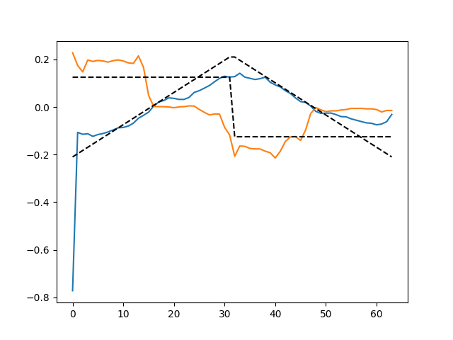
Note if the data is corrupted with impulsive noise, this method may not be the best. Check out our example using alphacsc to learn how to deal with such data.

alpha = 1.2
noise_level = 0.005
X[idx_corrupted] += levy_stable.rvs(alpha, 0, loc=0, scale=noise_level,
                                    size=(n_corrupted_trials, n_times),
                                    random_state=random_state_simulate)
pobj, times, d_hat, z_hat, reg = learn_d_z(
    X, n_atoms, n_times_atom, reg=reg, n_iter=n_iter,
    solver_d_kwargs=dict(factr=100), random_state=random_state,
    n_jobs=1, verbose=1)
plt.figure()
plt.plot(d_hat.T)
plt.plot(ds_true.T, 'k--')
plt.show()

Out:

V_0/50 .................................................

previous

Extracting cross-frequency coupling waveforms from rodent LFP data

next

Gait (steps) example