MoTIF on simulated data#

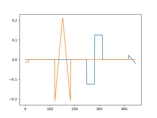
This example demonstrates MoTIF [1] on simulated data. In the alphacsc module, we are offering all the alternatives for the users to try. Please cite our paper [2] if you use this implementation.

[1] Jost, Philippe, et al.: “MoTIF: An efficient algorithm for learning translation invariant dictionaries.” Acoustics, Speech and Signal Processing, 2006. ICASSP 2006 Proceedings. 2006 IEEE International Conference on. Vol. 5. IEEE, 2006.
[2] Jas, M., Dupr’e La Tour, T., Simsekli, U., & Gramfort, A. (2017).: Learning the Morphology of Brain Signals Using Alpha-Stable Convolutional Sparse Coding. arXiv preprint arXiv:1705.08006.

# Authors: Mainak Jas <mainak.jas@telecom-paristech.fr>
#          Tom Dupre La Tour <tom.duprelatour@telecom-paristech.fr>
#          Umut Simsekli <umut.simsekli@telecom-paristech.fr>
#          Alexandre Gramfort <alexandre.gramfort@telecom-paristech.fr>
#
# License: BSD (3-clause)

Let us first import the modules.

import matplotlib.pyplot as plt
from alphacsc.simulate import simulate_data
from alphacsc.other.motif import learn_atoms

and define the relevant parameters. Note we choose a large n_times to avoid overlapping atoms which MoTIF cannot handle

n_times_atom = 64  # L
n_times = 5000  # T
n_atoms = 2  # K
n_trials = 10  # N

simulate the data.

random_state_simulate = 1
X, ds_true, z_true = simulate_data(n_trials, n_times, n_times_atom,
                                   n_atoms, random_state_simulate,
                                   constant_amplitude=True)

n_times_atom = n_times_atom * 7  # XXX: hack
n_iter = 10
max_shift = 11  # after this, the algorithm breaks

Note, how we use constant_amplitude=True since MoTIF cannot handle atoms of varying amplitudes. Check out our examples on vanilla CSC and alphaCSC to learn how to deal with such cases. Finally, let us estimate the atoms.

ds_hat = learn_atoms(X, n_atoms, n_times_atom, n_iter=n_iter,
                     max_shift=max_shift, random_state=42)
plt.plot(ds_hat.T)

Out:

/github/workspace/alphacsc/other/motif.py:34: DeprecationWarning: `np.int` is a deprecated alias for the builtin `int`. To silence this warning, use `int` by itself. Doing this will not modify any behavior and is safe. When replacing `np.int`, you may wish to use e.g. `np.int64` or `np.int32` to specify the precision. If you wish to review your current use, check the release note link for additional information.
Deprecated in NumPy 1.20; for more details and guidance: https://numpy.org/devdocs/release/1.20.0-notes.html#deprecations
  match = np.zeros((n_atoms, n_trials), dtype=np.int)
[seed 42] Atom 0 Iteration 0
[seed 42] Atom 0 Iteration 1
[seed 42] Atom 0 Iteration 2
[seed 42] Atom 0 Iteration 3
[seed 42] Atom 0 Iteration 4
[seed 42] Atom 0 Iteration 5
[seed 42] Atom 0 Iteration 6
[seed 42] Atom 0 Iteration 7
[seed 42] Atom 0 Iteration 8
[seed 42] Atom 0 Iteration 9
[seed 42] Atom 1 Iteration 0
[seed 42] Atom 1 Iteration 1
[seed 42] Atom 1 Iteration 2
[seed 42] Atom 1 Iteration 3
[seed 42] Atom 1 Iteration 4
[seed 42] Atom 1 Iteration 5
[seed 42] Atom 1 Iteration 6
[seed 42] Atom 1 Iteration 7
[seed 42] Atom 1 Iteration 8
[seed 42] Atom 1 Iteration 9

[<matplotlib.lines.Line2D object at 0x7f587ec65a60>, <matplotlib.lines.Line2D object at 0x7f587ec65640>]

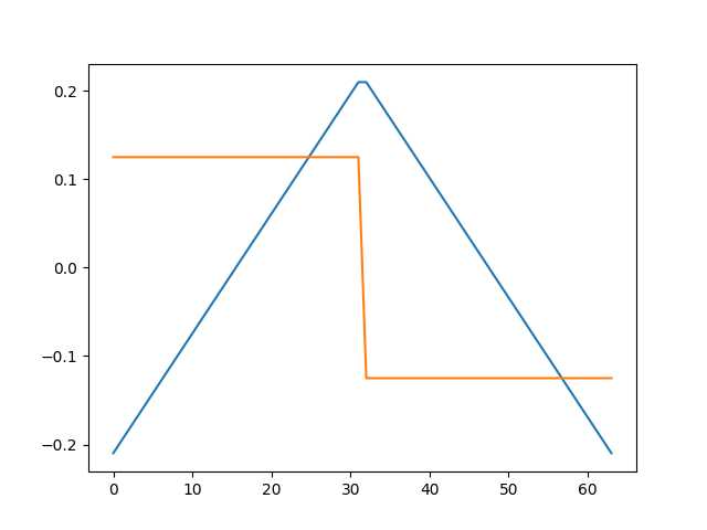
Compare this to the original atoms

plt.figure()
plt.plot(ds_true.T)
plt.show()

Total running time of the script: ( 0 minutes 0.572 seconds)

Gallery generated by Sphinx-Gallery

Alpha CSC on empirical time-series with strong artifacts

SWM on simulated data