Selecting random state for CSC

The CSC problem is non-convex. Therefore, the solution depends on the initialization. Here, we show how to select the best atoms amongst different initializations.

# Authors: Mainak Jas <mainak.jas@telecom-paristech.fr>
#          Tom Dupre La Tour <tom.duprelatour@telecom-paristech.fr>
#          Umut Simsekli <umut.simsekli@telecom-paristech.fr>
#          Alexandre Gramfort <alexandre.gramfort@telecom-paristech.fr>
#
# License: BSD (3-clause)

As before, let us first define the parameters of our model.

n_times_atom = 64  # L
n_times = 512  # T
n_atoms = 2  # K
n_trials = 100  # N
n_iter = 50

reg = 0.1

Here, we simulate the data

from alphacsc.simulate import simulate_data # noqa
from scipy.stats import levy_stable # noqa
from alphacsc import check_random_state # noqa

random_state_simulate = 1
X, ds_true, z_true = simulate_data(n_trials, n_times, n_times_atom,
                                   n_atoms, random_state_simulate)

# Add stationary noise:
fraction_corrupted = 0.02
n_corrupted_trials = int(fraction_corrupted * n_trials)

rng = check_random_state(random_state_simulate)
X += 0.01 * rng.randn(*X.shape)

idx_corrupted = rng.randint(0, n_trials,
                            size=n_corrupted_trials)

Now, we run vanilla CSC on the data but with different initializations.

from alphacsc import learn_d_z # noqa

pobjs, d_hats = list(), list()
for random_state in range(5):
    print('\nRandom state: %d' % random_state)
    pobj, times, d_hat, z_hat, reg = learn_d_z(
        X, n_atoms, n_times_atom, reg=reg, n_iter=n_iter,
        solver_d_kwargs=dict(factr=100), random_state=random_state,
        n_jobs=1, verbose=1)
    pobjs.append(pobj[-1])
    d_hats.append(d_hat)

Out:

Random state: 0
V_0/50 .................................................

Random state: 1
V_0/50 .................................................

Random state: 2
V_0/50 .................................................

Random state: 3
V_0/50 .................................................

Random state: 4
V_0/50 .................................................

As we loop through the random states, we save the objective value pobj at the last iteration of the algorithm.

Now, let us look at the atoms for different initializations.

import matplotlib.pyplot as plt # noqa
fig, axes = plt.subplots(1, 5, figsize=(17, 3), sharex=True, sharey=True)
for ax, this_pobjs, d_hat in zip(axes, pobjs, d_hats):
    ax.plot(d_hat.T)
    ax.plot(ds_true.T, 'k--')
    ax.set_title('pobj: %0.2f' % this_pobjs)

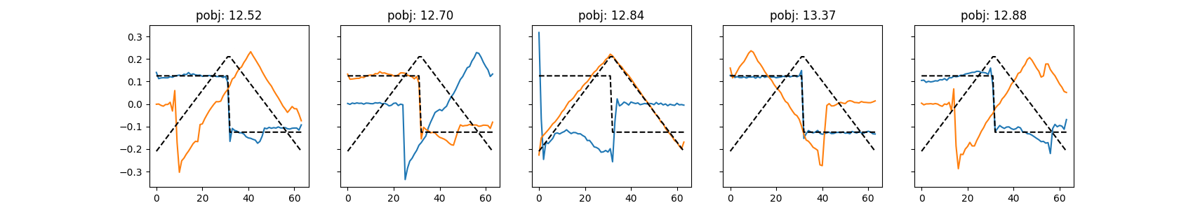
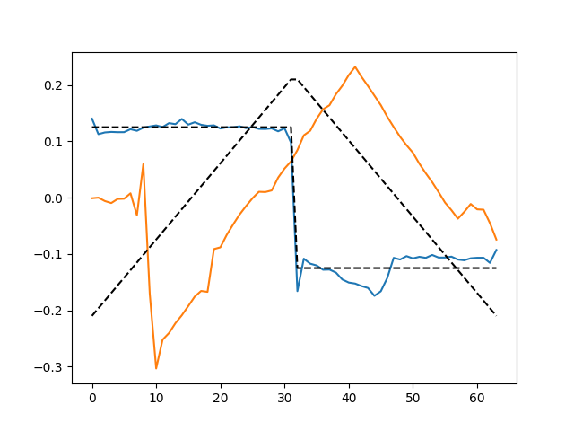
Note that lower the objective value, the better is the recovered atom. This is one reason why using a concrete mathematical objective function as in convolutional sparse coding is superior to heuristic methods. Now, we select the best atom amongst them.

import numpy as np # noqa

plt.figure()
plt.plot(d_hats[np.argmin(pobjs)].T)
plt.plot(ds_true.T, 'k--')
plt.show()

previous

Examples Gallery

next

CSC to learn LFP spiking atoms