Extracting cross-frequency coupling waveforms from rodent LFP data

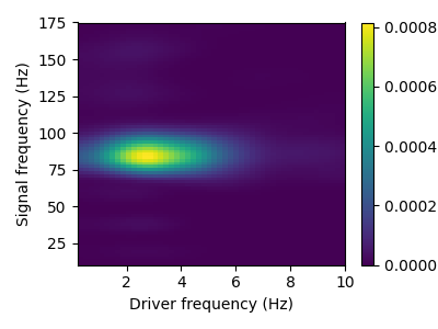
This example illustrates how to learn univariate atoms on a univariate time-serie. The data is a single LFP channel recorded on a rodent’s striatum [1]. Interestingly in this time-serie, the high frequency oscillations around 80 Hz are modulated in amplitude by the low-frequency oscillation around 3 Hz, a phenomenon known as cross-frequency coupling (CFC).

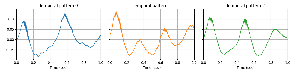
The convolutional sparse coding (CSC) model is able to learn the prototypical waveforms of the signal, on which we can clearly see the CFC.

[1]

G. Dallérac, M. Graupner, J. Knippenberg, R. C. R. Martinez, T. F. Tavares, L. Tallot, N. El Massioui, A. Verschueren, S. Höhn, J.B. Bertolus, et al. Updating temporal expectancy of an aversive event engages striatal plasticity under amygdala control. Nature Communications, 8:13920, 2017

# Authors: Tom Dupre La Tour <tom.duprelatour@telecom-paristech.fr>
#          Mainak Jas <mainak.jas@telecom-paristech.fr>
#          Umut Simsekli <umut.simsekli@telecom-paristech.fr>
#          Alexandre Gramfort <alexandre.gramfort@telecom-paristech.fr>
#
# License: BSD (3-clause)

Let us first load the data sample.

import mne
import numpy as np
import matplotlib.pyplot as plt

# sample frequency
sfreq = 350.

# We load the signal. It is an LFP channel recorded on a rodent's striatum.
data = np.load('../rodent_striatum.npy')
print(data.shape)

(1, 630000)

As the data contains severe artifacts between t=0 and t=100, we use a section not affected by artifacts.

data = data[:, 35000:]

# We also remove the slow drift, which accounts for a lot of variance.
data = mne.filter.filter_data(data, sfreq, 1, None)

# To make the most of parallel computing, we split the data into trials.
data = data.reshape(50, -1)
data /= data.std()

Setting up high-pass filter at 1 Hz

FIR filter parameters
---------------------
Designing a one-pass, zero-phase, non-causal highpass filter:
- Windowed time-domain design (firwin) method
- Hamming window with 0.0194 passband ripple and 53 dB stopband attenuation
- Lower passband edge: 1.00
- Lower transition bandwidth: 1.00 Hz (-6 dB cutoff frequency: 0.50 Hz)
- Filter length: 1155 samples (3.300 s)

This sample contains CFC between 3 Hz and 80 Hz. This phenomenon can be described with a comodulogram, computed for instance with the pactools Python library.

from pactools import Comodulogram

comod = Comodulogram(fs=sfreq, low_fq_range=np.arange(0.2, 10.2, 0.2),
                     low_fq_width=2., method='duprelatour')
comod.fit(data)
comod.plot()
plt.show()

[                                        ] 0% | 0.00 sec | comodulogram: DAR(10, 1)
[                                        ] 2% | 0.57 sec | comodulogram: DAR(10, 1)
[.                                       ] 4% | 0.90 sec | comodulogram: DAR(10, 1)
[..                                      ] 6% | 1.23 sec | comodulogram: DAR(10, 1)
[...                                     ] 8% | 1.56 sec | comodulogram: DAR(10, 1)
[....                                    ] 10% | 1.89 sec | comodulogram: DAR(10, 1)
[....                                    ] 12% | 2.24 sec | comodulogram: DAR(10, 1)
[.....                                   ] 14% | 2.57 sec | comodulogram: DAR(10, 1)
[......                                  ] 16% | 2.91 sec | comodulogram: DAR(10, 1)
[.......                                 ] 18% | 3.25 sec | comodulogram: DAR(10, 1)
[........                                ] 20% | 3.56 sec | comodulogram: DAR(10, 1)
[........                                ] 22% | 3.90 sec | comodulogram: DAR(10, 1)
[.........                               ] 24% | 4.25 sec | comodulogram: DAR(10, 1)
[..........                              ] 26% | 4.58 sec | comodulogram: DAR(10, 1)
[...........                             ] 28% | 4.90 sec | comodulogram: DAR(10, 1)
[............                            ] 30% | 5.24 sec | comodulogram: DAR(10, 1)
[............                            ] 32% | 5.58 sec | comodulogram: DAR(10, 1)
[.............                           ] 34% | 5.92 sec | comodulogram: DAR(10, 1)
[..............                          ] 36% | 6.24 sec | comodulogram: DAR(10, 1)
[...............                         ] 38% | 6.55 sec | comodulogram: DAR(10, 1)
[................                        ] 40% | 6.89 sec | comodulogram: DAR(10, 1)
[................                        ] 42% | 7.23 sec | comodulogram: DAR(10, 1)
[.................                       ] 44% | 7.54 sec | comodulogram: DAR(10, 1)
[..................                      ] 46% | 7.88 sec | comodulogram: DAR(10, 1)
[...................                     ] 48% | 8.22 sec | comodulogram: DAR(10, 1)
[....................                    ] 50% | 8.52 sec | comodulogram: DAR(10, 1)
[....................                    ] 52% | 8.83 sec | comodulogram: DAR(10, 1)
[.....................                   ] 54% | 9.14 sec | comodulogram: DAR(10, 1)
[......................                  ] 56% | 9.47 sec | comodulogram: DAR(10, 1)
[.......................                 ] 58% | 9.78 sec | comodulogram: DAR(10, 1)
[........................                ] 60% | 10.10 sec | comodulogram: DAR(10, 1)
[........................                ] 62% | 10.40 sec | comodulogram: DAR(10, 1)
[.........................               ] 64% | 10.71 sec | comodulogram: DAR(10, 1)
[..........................              ] 66% | 11.02 sec | comodulogram: DAR(10, 1)
[...........................             ] 68% | 11.32 sec | comodulogram: DAR(10, 1)
[............................            ] 70% | 11.62 sec | comodulogram: DAR(10, 1)
[............................            ] 72% | 11.92 sec | comodulogram: DAR(10, 1)
[.............................           ] 74% | 12.22 sec | comodulogram: DAR(10, 1)
[..............................          ] 76% | 12.53 sec | comodulogram: DAR(10, 1)
[...............................         ] 78% | 12.83 sec | comodulogram: DAR(10, 1)
[................................        ] 80% | 13.14 sec | comodulogram: DAR(10, 1)
[................................        ] 82% | 13.44 sec | comodulogram: DAR(10, 1)
[.................................       ] 84% | 13.74 sec | comodulogram: DAR(10, 1)
[..................................      ] 86% | 14.05 sec | comodulogram: DAR(10, 1)
[...................................     ] 88% | 14.36 sec | comodulogram: DAR(10, 1)
[....................................    ] 90% | 14.66 sec | comodulogram: DAR(10, 1)
[....................................    ] 92% | 14.96 sec | comodulogram: DAR(10, 1)
[.....................................   ] 94% | 15.24 sec | comodulogram: DAR(10, 1)
[......................................  ] 96% | 15.54 sec | comodulogram: DAR(10, 1)
[....................................... ] 98% | 15.85 sec | comodulogram: DAR(10, 1)
[........................................] 100% | 16.16 sec | comodulogram: DAR(10, 1)

[........................................] 100% | 16.16 sec | comodulogram: DAR(10, 1)

We fit a CSC model on the data.

from alphacsc import learn_d_z

params = dict(
    n_atoms=3,
    n_times_atom=int(sfreq * 1.0),  # 1000. ms
    reg=5.,
    n_iter=10,
    solver_z='l-bfgs',
    solver_z_kwargs=dict(factr=1e9),
    solver_d_kwargs=dict(factr=1e2),
    random_state=42,
    n_jobs=5,
    verbose=1)

_, _, d_hat, z_hat, _ = learn_d_z(data, **params)

V_0/10 /github/workspace/alphacsc/update_d.py:224: DeprecationWarning: Conversion of an array with ndim > 0 to a scalar is deprecated, and will error in future. Ensure you extract a single element from your array before performing this operation. (Deprecated NumPy 1.25.)
  lhs_c_copy[0] += lambd
/github/workspace/alphacsc/update_d.py:172: DeprecationWarning: Conversion of an array with ndim > 0 to a scalar is deprecated, and will error in future. Ensure you extract a single element from your array before performing this operation. (Deprecated NumPy 1.25.)
  lambd_hats[k] = lambd_hat
.........

Plot the temporal patterns. Interestingly, we obtain prototypical waveforms of the signal on which we can clearly see the CFC.

n_atoms, n_times_atom = d_hat.shape
n_columns = min(6, n_atoms)
n_rows = int(np.ceil(n_atoms // n_columns))
figsize = (4 * n_columns, 3 * n_rows)
fig, axes = plt.subplots(n_rows, n_columns, figsize=figsize, sharey=True)
axes = axes.ravel()

for kk in range(n_atoms):
    ax = axes[kk]
    time = np.arange(n_times_atom) / sfreq
    ax.plot(time, d_hat[kk], color='C%d' % kk)
    ax.set_xlim(0, n_times_atom / sfreq)
    ax.set(xlabel='Time (sec)', title="Temporal pattern %d" % kk)
    ax.grid(True)

fig.tight_layout()
plt.show()