Alpha CSC on simulated data

This example demonstrates alphaCSC 1 on simulated data.

1

Jas, M., Dupré La Tour, T., Şimşekli, U., & Gramfort, A. (2017). Learning the Morphology of Brain Signals Using Alpha-Stable Convolutional Sparse Coding. Advances in Neural Information Processing Systems (NIPS), pages 1099–1108.

# Authors: Mainak Jas <mainak.jas@telecom-paristech.fr>
#          Tom Dupre La Tour <tom.duprelatour@telecom-paristech.fr>
#          Umut Simsekli <umut.simsekli@telecom-paristech.fr>
#          Alexandre Gramfort <alexandre.gramfort@telecom-paristech.fr>
#
# License: BSD (3-clause)

Let us first define the parameters of our model.

n_times_atom = 64  # L
n_times = 512  # T
n_atoms = 2  # K
n_trials = 100  # N

alpha = 1.2
reg = 0.1

Next, we define the parameters for alpha CSC

n_iter_global = 10
n_iter_optim = 50
n_iter_mcmc = 100
n_burnin_mcmc = 50

Here, we simulate the data

from alphacsc.simulate import simulate_data

random_state_simulate = 1
X, ds_true, z_true = simulate_data(n_trials, n_times, n_times_atom,
                                   n_atoms, random_state_simulate)

Add some noise and corrupt some trials even with impulsive noise

from scipy.stats import levy_stable
from alphacsc import check_random_state

fraction_corrupted = 0.02
n_corrupted_trials = int(fraction_corrupted * n_trials)

# Add stationary noise:
rng = check_random_state(random_state_simulate)
X += 0.01 * rng.randn(*X.shape)

noise_level = 0.005
# add impulsive noise
idx_corrupted = rng.randint(0, n_trials,
                            size=n_corrupted_trials)
X[idx_corrupted] += levy_stable.rvs(alpha, 0, loc=0, scale=noise_level,
                                    size=(n_corrupted_trials, n_times),
                                    random_state=random_state_simulate)

and then alpha CSC on the same data

from alphacsc import learn_d_z_weighted

d_hat, z_hat, Tau = learn_d_z_weighted(
    X, n_atoms, n_times_atom, reg=reg, alpha=alpha,
    solver_d_kwargs=dict(factr=100), n_iter_global=n_iter_global,
    n_iter_optim=n_iter_optim, init_tau=True,
    n_iter_mcmc=n_iter_mcmc, n_burnin_mcmc=n_burnin_mcmc,
    random_state=60, n_jobs=1, verbose=1)

Out:

Global Iter: 0/10       V_0/50 .................................................
Global Iter: 1/10       V_0/50 .................................................
Global Iter: 2/10       V_0/50 .................................................
Global Iter: 3/10       V_0/50 .................................................
Global Iter: 4/10       V_0/50 .................................................
Global Iter: 5/10       V_0/50 .................................................
Global Iter: 6/10       V_0/50 .................................................
Global Iter: 7/10       V_0/50 .................................................
Global Iter: 8/10       V_0/50 .................................................
Global Iter: 9/10       V_0/50 .................................................

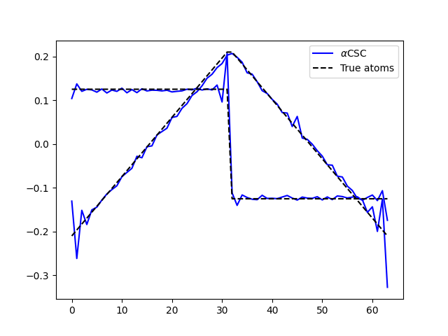
Finally, let’s compare the results. Now, it works even in the presence of impulsive noise.

import matplotlib.pyplot as plt

plt.figure()
plt.plot(d_hat.T, 'b', label=r'$\alpha$CSC')
plt.plot(ds_true.T, 'k--', label='True atoms')
handles, labels = plt.gca().get_legend_handles_labels()
plt.legend(handles[::2], labels[::2], loc='best')
plt.show()

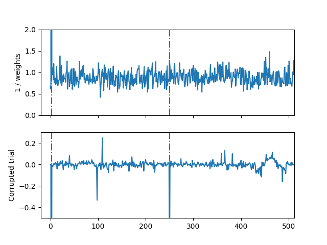
We can even visualize the weights to see what time points were downweighted by the algorithm

fig, axes = plt.subplots(2, 1, sharex=True)
axes[0].set_xlim([-20, n_times])
axes[0].set_ylim([0, 2])
axes[1].set_ylim([-0.5, 0.3])

for t in [2, 250]:
    axes[0].axvline(t, linestyle='-.')
    axes[1].axvline(t, linestyle='-.')

axes[0].plot(1 / Tau[idx_corrupted[0], :])
axes[0].set_ylabel('1 / weights')
axes[1].plot(X[idx_corrupted[0], :])
axes[1].set_ylabel('Corrupted trial')

Out:

Text(31.222222222222214, 0.5, 'Corrupted trial')

previous

Extracting artifact and evoked response atoms from the sample dataset

next

Alpha CSC on empirical time-series with strong artifacts