Note
Go to the end to download the full example code.
Extracting \(\mu\)-wave from the somato-sensory dataset#
This example illustrates how to learn rank-1 atoms [1] on the multivariate
somato-sensorymotor dataset from mne. The displayed results highlight
the presence of \(\mu\)-waves located in the SI cortex.
# Authors: Thomas Moreau <thomas.moreau@inria.fr>
#          Mainak Jas <mainak.jas@telecom-paristech.fr>
#          Tom Dupre La Tour <tom.duprelatour@telecom-paristech.fr>
#          Alexandre Gramfort <alexandre.gramfort@telecom-paristech.fr>
#
# License: BSD (3-clause)
Let us first define the parameters of our model.
sfreq = 150.

# Define the shape of the dictionary
n_atoms = 25
n_times_atom = int(round(sfreq * 1.0))  # 1000. ms
Next, we define the parameters for multivariate CSC
from alphacsc import BatchCDL
cdl = BatchCDL(
    # Shape of the dictionary
    n_atoms=n_atoms,
    n_times_atom=n_times_atom,
    # Request a rank1 dictionary with unit norm temporal and spatial maps
    rank1=True, uv_constraint='separate',
    # Initialize the dictionary with random chunk from the data
    D_init='chunk',
    # rescale the regularization parameter to be 20% of lambda_max
    lmbd_max="scaled", reg=.2,
    # Number of iteration for the alternate minimization and cvg threshold
    n_iter=100, eps=1e-4,
    # solver for the z-step
    solver_z="lgcd", solver_z_kwargs={'tol': 1e-2, 'max_iter': 1000},
    # solver for the d-step
    solver_d='alternate_adaptive', solver_d_kwargs={'max_iter': 300},
    # Technical parameters
    verbose=1, random_state=0, n_jobs=6)
Here, we load the data from the somato-sensory dataset and preprocess them in epochs. The epochs are selected around the stim, starting 2 seconds before and finishing 4 seconds after.
Using default location ~/mne_data for somato...

  0%|                                               | 0.00/611M [00:00<?, ?B/s]
  0%|▏                                     | 2.63M/611M [00:00<00:23, 26.3MB/s]
  2%|▌                                     | 10.0M/611M [00:00<00:11, 54.3MB/s]
  3%|█                                     | 17.4M/611M [00:00<00:09, 63.0MB/s]
  4%|█▌                                    | 24.7M/611M [00:00<00:08, 67.0MB/s]
  5%|█▉                                    | 32.1M/611M [00:00<00:08, 69.5MB/s]
  6%|██▍                                   | 39.4M/611M [00:00<00:08, 70.7MB/s]
  8%|██▉                                   | 46.4M/611M [00:00<00:08, 70.0MB/s]
  9%|███▎                                  | 53.7M/611M [00:00<00:07, 70.9MB/s]
 10%|███▊                                  | 61.0M/611M [00:00<00:07, 71.3MB/s]
 11%|████▎                                 | 68.3M/611M [00:01<00:07, 72.1MB/s]
 12%|████▋                                 | 75.6M/611M [00:01<00:07, 72.3MB/s]
 14%|█████▏                                | 82.9M/611M [00:01<00:07, 72.1MB/s]
 15%|█████▌                                | 90.2M/611M [00:01<00:07, 72.5MB/s]
 16%|██████                                | 97.4M/611M [00:01<00:07, 72.4MB/s]
 17%|██████▋                                | 105M/611M [00:01<00:07, 72.1MB/s]
 18%|███████▏                               | 112M/611M [00:01<00:06, 72.3MB/s]
 20%|███████▌                               | 119M/611M [00:01<00:06, 72.2MB/s]
 21%|████████                               | 126M/611M [00:01<00:06, 72.3MB/s]
 22%|████████▌                              | 134M/611M [00:01<00:06, 72.7MB/s]
 23%|█████████                              | 141M/611M [00:02<00:06, 72.9MB/s]
 24%|█████████▍                             | 148M/611M [00:02<00:06, 73.0MB/s]
 26%|█████████▉                             | 156M/611M [00:02<00:06, 73.0MB/s]
 27%|██████████▍                            | 163M/611M [00:02<00:06, 73.1MB/s]
 28%|██████████▉                            | 170M/611M [00:02<00:06, 73.3MB/s]
 29%|███████████▎                           | 178M/611M [00:02<00:05, 73.2MB/s]
 30%|███████████▊                           | 185M/611M [00:02<00:05, 72.9MB/s]
 32%|████████████▎                          | 192M/611M [00:02<00:05, 72.7MB/s]
 33%|████████████▊                          | 200M/611M [00:02<00:05, 72.6MB/s]
 34%|█████████████▏                         | 207M/611M [00:02<00:05, 72.7MB/s]
 35%|█████████████▋                         | 214M/611M [00:03<00:05, 72.5MB/s]
 36%|██████████████▏                        | 222M/611M [00:03<00:05, 72.6MB/s]
 37%|██████████████▌                        | 229M/611M [00:03<00:05, 72.7MB/s]
 39%|███████████████                        | 236M/611M [00:03<00:05, 73.0MB/s]
 40%|███████████████▌                       | 244M/611M [00:03<00:05, 73.1MB/s]
 41%|████████████████                       | 251M/611M [00:03<00:04, 73.7MB/s]
 42%|████████████████▌                      | 259M/611M [00:03<00:04, 74.0MB/s]
 44%|████████████████▉                      | 266M/611M [00:03<00:04, 74.3MB/s]
 45%|█████████████████▍                     | 274M/611M [00:03<00:04, 74.6MB/s]
 46%|█████████████████▉                     | 281M/611M [00:03<00:04, 74.6MB/s]
 47%|██████████████████▍                    | 288M/611M [00:04<00:04, 74.4MB/s]
 48%|██████████████████▉                    | 296M/611M [00:04<00:04, 73.7MB/s]
 50%|███████████████████▍                   | 303M/611M [00:04<00:04, 73.6MB/s]
 51%|███████████████████▊                   | 311M/611M [00:04<00:04, 73.2MB/s]
 52%|████████████████████▎                  | 318M/611M [00:04<00:03, 73.5MB/s]
 53%|████████████████████▊                  | 326M/611M [00:04<00:03, 74.0MB/s]
 55%|█████████████████████▎                 | 333M/611M [00:04<00:03, 74.3MB/s]
 56%|█████████████████████▊                 | 341M/611M [00:04<00:03, 74.4MB/s]
 57%|██████████████████████▏                | 348M/611M [00:04<00:03, 74.7MB/s]
 58%|██████████████████████▋                | 356M/611M [00:04<00:03, 74.7MB/s]
 59%|███████████████████████▏               | 363M/611M [00:05<00:03, 74.9MB/s]
 61%|███████████████████████▋               | 371M/611M [00:05<00:03, 75.7MB/s]
 62%|████████████████████████▏              | 378M/611M [00:05<00:03, 64.6MB/s]
 63%|████████████████████████▌              | 385M/611M [00:05<00:03, 65.4MB/s]
 64%|█████████████████████████              | 392M/611M [00:05<00:03, 67.5MB/s]
 65%|█████████████████████████▌             | 400M/611M [00:05<00:03, 68.7MB/s]
 67%|█████████████████████████▉             | 407M/611M [00:05<00:02, 69.9MB/s]
 68%|██████████████████████████▍            | 414M/611M [00:05<00:02, 70.7MB/s]
 69%|██████████████████████████▉            | 422M/611M [00:05<00:02, 71.3MB/s]
 70%|███████████████████████████▍           | 429M/611M [00:05<00:02, 71.8MB/s]
 71%|███████████████████████████▊           | 436M/611M [00:06<00:02, 72.0MB/s]
 73%|████████████████████████████▎          | 443M/611M [00:06<00:02, 72.1MB/s]
 74%|████████████████████████████▊          | 451M/611M [00:06<00:02, 72.2MB/s]
 75%|█████████████████████████████▏         | 458M/611M [00:06<00:02, 72.2MB/s]
 76%|█████████████████████████████▋         | 465M/611M [00:06<00:02, 72.2MB/s]
 77%|██████████████████████████████▏        | 472M/611M [00:06<00:01, 72.3MB/s]
 79%|██████████████████████████████▋        | 480M/611M [00:06<00:01, 72.4MB/s]
 80%|███████████████████████████████        | 487M/611M [00:06<00:01, 72.2MB/s]
 81%|███████████████████████████████▌       | 494M/611M [00:06<00:01, 72.3MB/s]
 82%|████████████████████████████████       | 501M/611M [00:06<00:01, 72.4MB/s]
 83%|████████████████████████████████▍      | 509M/611M [00:07<00:01, 72.4MB/s]
 84%|████████████████████████████████▉      | 516M/611M [00:07<00:01, 72.4MB/s]
 86%|█████████████████████████████████▍     | 523M/611M [00:07<00:01, 72.6MB/s]
 87%|█████████████████████████████████▉     | 530M/611M [00:07<00:01, 72.5MB/s]
 88%|██████████████████████████████████▎    | 538M/611M [00:07<00:01, 72.5MB/s]
 89%|██████████████████████████████████▊    | 545M/611M [00:07<00:00, 72.3MB/s]
 90%|███████████████████████████████████▎   | 552M/611M [00:07<00:00, 72.1MB/s]
 92%|███████████████████████████████████▋   | 559M/611M [00:07<00:00, 71.8MB/s]
 93%|████████████████████████████████████▏  | 566M/611M [00:07<00:00, 71.8MB/s]
 94%|████████████████████████████████████▋  | 574M/611M [00:07<00:00, 71.9MB/s]
 95%|█████████████████████████████████████  | 581M/611M [00:08<00:00, 71.8MB/s]
 96%|█████████████████████████████████████▌ | 588M/611M [00:08<00:00, 71.7MB/s]
 98%|██████████████████████████████████████ | 595M/611M [00:08<00:00, 71.9MB/s]
 99%|██████████████████████████████████████▍| 603M/611M [00:08<00:00, 72.1MB/s]
100%|██████████████████████████████████████▉| 610M/611M [00:08<00:00, 72.9MB/s]
  0%|                                               | 0.00/611M [00:00<?, ?B/s]
100%|███████████████████████████████████████| 611M/611M [00:00<00:00, 4.07TB/s]
/usr/local/lib/python3.13/site-packages/pooch/processors.py:262: DeprecationWarning: Python 3.14 will, by default, filter extracted tar archives and reject files or modify their metadata. Use the filter argument to control this behavior.
  tar_file.extractall(path=extract_dir)
Attempting to create new mne-python configuration file:
/github/home/.mne/mne-python.json
Could not read the /github/home/.mne/mne-python.json json file during the writing. Assuming it is empty. Got: Expecting value: line 1 column 1 (char 0)
Download complete in 18s (582.2 MB)
Opening raw data file /github/home/mne_data/MNE-somato-data/sub-01/meg/sub-01_task-somato_meg.fif...
    Range : 237600 ... 506999 =    791.189 ...  1688.266 secs
Ready.
Reading 0 ... 269399  =      0.000 ...   897.077 secs...
Filtering raw data in 1 contiguous segment
Setting up band-stop filter

FIR filter parameters
---------------------
Designing a one-pass, zero-phase, non-causal bandstop filter:
- Windowed time-domain design (firwin) method
- Hamming window with 0.0194 passband ripple and 53 dB stopband attenuation
- Lower transition bandwidth: 0.50 Hz
- Upper transition bandwidth: 0.50 Hz
- Filter length: 1983 samples (6.603 s)

Filtering raw data in 1 contiguous segment
Setting up high-pass filter at 2 Hz

FIR filter parameters
---------------------
Designing a one-pass, zero-phase, non-causal highpass filter:
- Windowed time-domain design (firwin) method
- Hamming window with 0.0194 passband ripple and 53 dB stopband attenuation
- Lower passband edge: 2.00
- Lower transition bandwidth: 2.00 Hz (-6 dB cutoff frequency: 1.00 Hz)
- Filter length: 497 samples (1.655 s)

Finding events on: STI 014
111 events found on stim channel STI 014
Event IDs: [1]
Not setting metadata
111 matching events found
Setting baseline interval to [-3.9992341833870637, 0.0] s
Applying baseline correction (mode: mean)
0 projection items activated
Using data from preloaded Raw for 111 events and 1202 original time points ...
    Rejecting  epoch based on EOG : ['EOG 061']
    Rejecting  epoch based on EOG : ['EOG 061']
    Rejecting  epoch based on EOG : ['EOG 061']
    Rejecting  epoch based on EOG : ['EOG 061']
    Rejecting  epoch based on EOG : ['EOG 061']
5 bad epochs dropped
NOTE: pick_types() is a legacy function. New code should use inst.pick(...).
/github/workspace/alphacsc/datasets/mne_data.py:98: RuntimeWarning: Something went wrong in the data-driven estimation of the data rank as it exceeds the theoretical rank from the info (204 > 64). Consider setting rank to "auto" or setting it explicitly as an integer.
  cov = mne.compute_covariance(epochs_cov)
Reducing data rank from 204 -> 204
Estimating covariance using EMPIRICAL
Done.
Number of samples used : 127412
[done]
Not setting metadata
111 matching events found
Setting baseline interval to [-2.001282051803185, 0.0] s
Applying baseline correction (mode: mean)
0 projection items activated
Using data from preloaded Raw for 111 events and 1803 original time points ...
    Rejecting  epoch based on EOG : ['EOG 061']
    Rejecting  epoch based on EOG : ['EOG 061']
    Rejecting  epoch based on EOG : ['EOG 061']
    Rejecting  epoch based on EOG : ['EOG 061']
    Rejecting  epoch based on EOG : ['EOG 061']
    Rejecting  epoch based on EOG : ['EOG 061']
    Rejecting  epoch based on EOG : ['EOG 061']
    Rejecting  epoch based on EOG : ['EOG 061']
8 bad epochs dropped
NOTE: pick_types() is a legacy function. New code should use inst.pick(...).
Fit the model and learn rank1 atoms
..............
[BatchCDL] Fit in 352.9s

<alphacsc.convolutional_dictionary_learning.BatchCDL object at 0x7f33fc5cc550>
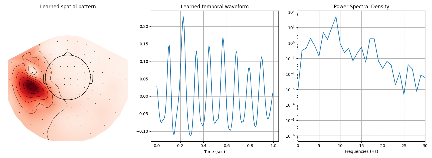
Display the 4-th atom, which displays a \(\mu\)-waveform in its temporal pattern.
import mne
import numpy as np
import matplotlib.pyplot as plt

i_atom = 4
n_plots = 3
figsize = (n_plots * 5, 5.5)
fig, axes = plt.subplots(1, n_plots, figsize=figsize, squeeze=False)

# Plot the spatial map of the learn atom using mne topomap
ax = axes[0, 0]
u_hat = cdl.u_hat_[i_atom]
mne.viz.plot_topomap(u_hat, info, axes=ax, show=False)
ax.set(title='Learned spatial pattern')

# Plot the temporal pattern of the learn atom
ax = axes[0, 1]
v_hat = cdl.v_hat_[i_atom]
t = np.arange(v_hat.size) / sfreq
ax.plot(t, v_hat)
ax.set(xlabel='Time (sec)', title='Learned temporal waveform')
ax.grid(True)

# Plot the psd of the time atom
ax = axes[0, 2]
psd = np.abs(np.fft.rfft(v_hat)) ** 2
frequencies = np.linspace(0, sfreq / 2.0, len(psd))
ax.semilogy(frequencies, psd)
ax.set(xlabel='Frequencies (Hz)', title='Power Spectral Density')
ax.grid(True)
ax.set_xlim(0, 30)

plt.tight_layout()
plt.show()
Total running time of the script: (6 minutes 20.268 seconds)